Regression analysis (mqr.plot.regression)

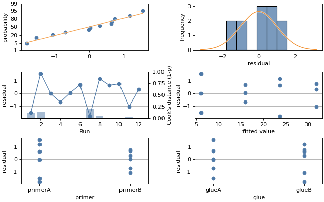
residuals(resid, fitted, axs)	Plot a probability plot of residuals, histogram of residuals, residuals versus observation and residuals versus fitted values for the residuals in a fitted statsmodels model.
influence(result, influence_stat, ax[, bar_kws])	Plot a bar graph of an influence statistic onto a twin axis of ax.
res_probplot(resid, ax[, probplot_kws])	Probability plot of residuals from result of calling fit() on statsmodels model.
res_histogram(resid, ax[, show_density, ...])	Plot histogram of residuals from result of calling fit() on statsmodels model.
res_v_obs(resid, ax[, plot_kws, bar_kws])	Plot residuals versus observations.
res_v_fit(resid, fitted, ax[, plot_kws])	Plot residual versus fit.
res_v_factor(resid, factor, ax[, ...])	Plot a factor versus fit.

Examples

This example uses residuals which displays res_probplot, res_histogram, res_v_obs and res_v_fit into four supplied axes. The example also plots th residuals against factors using res_v_factor. Finally, the example overlay on the res_v_obs plot an influence statistic using influence.

First set up the data and fit a model whose residuals will be shown.

import statsmodels

# Raw data
data = pd.read_csv(mqr.sample_data('anova-glue.csv'), index_col='Run')

# Fit a linear model
model = statsmodels.formula.api.ols('adhesion_force ~ C(primer) * C(glue)', data)
result = model.fit()

(Source code)

Now create the residuals plots. There are six axes altogether: four for residuals and another two for res_v_factor applied to each factor.

fig, axs = plt.subplots(3, 2, figsize=(8, 5), layout='constrained')

# show the four residuals plots
mqr.plot.regression.residuals(result.resid, result.fittedvalues, axs=axs[:2, :])

# plot residuals against each factor
mqr.plot.regression.res_v_factor(result.resid, data['primer'], axs[2, 0])
mqr.plot.regression.res_v_factor(result.resid, data['glue'], axs[2, 1])

# show Cook's Distance measure of influence.
mqr.plot.regression.influence(result, 'cooks_dist', axs[1, 0])

(Source code, png, pdf)