mqr.plot.msa.

grr#

mqr.plot.msa.grr(grr, axs, sources=None)#

GRR summary plots.

A 3 by 2 grid of:

bar graph of components of variation,
measurement by part,
R-chart by operator,
measurement by operator,
Xbar-chart by operator, and
part * operator interaction.

This routine flattens the axes before drawing into them.

Parameters:

grrmqr.msa.GRR: GRR study.
axsnumpy.ndarray: A 3*2 array of matplotlib axes.
sourceslist[str], optional: A list of components of variation to include in the bar graph (optional).

Examples

Create plots for a GRR analysis from the NIST silicon wafer resistivity. Data is from https://www.itl.nist.gov/div898/software/dataplot/data/MPC61.DAT.

Before creating the plot, though, there is a bit of data marshalling to do. This loads the data from the CSV file online into a DataFrame. The first 50 rows are metadata etc., so skip those. Treat any one or more whitespace characters as a separator. And finally, add a column assigning numbers to repeated measurements, which allows the GRR routines to include repeats in the linear model.

columns = ['RUNID', 'WAFERID', 'PROBE', 'MONTH', 'DAY', 'OPERATOR', 'TEMP', 'AVERAGE', 'STDDEV',]
dtype = {
    'WAFERID': int,
    'PROBE':int,
}

data = pd.read_csv(
    'https://www.itl.nist.gov/div898/software/dataplot/data/MPC61.DAT',
    skiprows=50,
    header=None,
    names=columns,
    sep='\\s+',
    dtype=dtype,
    storage_options={'user-agent': 'github:nklsxn/mqr'}
)
data['REPEAT'] = np.repeat([1,2,3,4,5,6,7,8,9,10,11,12], 25)

(Source code)

The GRR plots are created from a GRR study object mqr.msa.GRR. For this example, use a tolerance of 8 ohm cm, and test for variance contribution from the probe (listed as operator). The name mapping shows the setup. This study uses only the first run RUNID == 1.

tol = 2*8.0
names = mqr.msa.NameMapping(
    part='WAFERID',
    operator='PROBE',
    measurement='AVERAGE')
grr = mqr.msa.GRR(
    data.query('RUNID==1'),
    tolerance=tol,
    names=names,
    include_interaction=True)

fig, axs = plt.subplots(3, 2, figsize=(10, 6), layout='constrained')
mqr.plot.msa.grr(grr, axs=axs)

(Source code, png, pdf)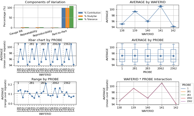