Statistical Process Control#
- Related modules
mqr.spc(andmqr.plot.spc)- Detailed examples
MQR provides classes for statistical process control. While the tools are designed for use with the plotting functions, they can also be used independently of control charts, for example in scripts that detect alarm conditions and take some automated action like sending an email, displaying on a dashboard, etc.
Background#
Traditionally, charts based on range and standard deviation have been defined and used together. For example, X-bar and R charts (both based on sample range) are often defined together. In this module, charts are treated separately so that XBarParams is used with R and S charts. XBarParams has methods to construct its parameters from either range or standard deviation.
When control charts were originally developed, they were drawn by hand. To make drawing practical, the historical chart parameters (control, upper and lower limits) were defined in terms of tabulated constants. For example, the upper control limit of an XBar chart that was based on the sample range was often written with a constant \(A_2\) as \(\mathrm{UCL} = \overline{\overline{x}} + A_2 \overline{R}\), where \(A_2\) is \(3/(d_2(n)\sqrt{n})\), which includes a factor to estimate process standard deviation from sample range (\(1 / d_2(n)\)), the scale of the standard error of the mean (\(1 / \sqrt{n}\)), and the width of the limits (\(3\) standard errors). Since this library plots charts automatically, it does not use or provide a way to calculate those traditional constants. Instead, it calculates all parameters directly, using lookup tables for pre-calculated unbiasing constants.
If necessary, the traditional constants are easy to calculate from standard errors
and the unbiasing constants implemented in MQR (see mqr.spc.util).
For details on those traditional parameters, see [1].
Data Handling#
The routines in mqr.spc expect sample data to be passed in a particular way.
For now, all sample sizes must be the same, though the sample sizes used to construct parameters
need not match the size of the samples used to monitor a process in production —
their standard errors are calculated separately.
Data should be formatted into pandas DataFrames with sample labels in the index.
That is, if a process is sampled twice per day, then the first sample on the first day
would be in the first row, the second sample that afternoon would be in the second row,
the sample from the next morning would be in row three, and so on.
Data should be formatted as follows.
For XBarParams, RParams, SParams and EwmaParams each column corresponds to an observation in a sample.
For MewmaParams each column corresponds to a measurements from a dimensions/KPIs.
This sample data is provided with MQR. It is the format that should be used with XBarParams, RParams, etc. It shows 20 samples labelled from “0” to “19” in the index. Each sample has eight observations labelled in the columns as “x1” to “x8”.
pd.read_csv(mqr.sample_data('spc.csv'))
| x1 | x2 | x3 | x4 | x5 | x6 | x7 | x8 | |
|---|---|---|---|---|---|---|---|---|
| 0 | 9.9976 | 10.0021 | 9.9961 | 9.9986 | 10.0033 | 9.9979 | 10.0026 | 9.9983 |
| 1 | 9.9998 | 10.0004 | 10.0006 | 9.9976 | 10.0017 | 10.0021 | 10.0025 | 9.9999 |
| 2 | 9.9998 | 9.9987 | 9.9972 | 9.9992 | 9.9990 | 9.9996 | 9.9988 | 10.0037 |
| 3 | 10.0005 | 9.9977 | 9.9963 | 9.9984 | 10.0028 | 10.0021 | 9.9999 | 9.9993 |
| 4 | 9.9963 | 9.9986 | 10.0024 | 9.9984 | 10.0008 | 9.9977 | 9.9968 | 9.9977 |
| 5 | 10.0014 | 9.9990 | 9.9978 | 10.0045 | 9.9968 | 10.0014 | 9.9966 | 9.9980 |
| 6 | 10.0009 | 10.0046 | 9.9982 | 10.0009 | 10.0033 | 10.0010 | 9.9976 | 9.9990 |
| 7 | 9.9994 | 10.0001 | 10.0018 | 9.9993 | 10.0005 | 9.9973 | 9.9995 | 9.9996 |
| 8 | 9.9981 | 9.9998 | 9.9992 | 9.9981 | 9.9992 | 10.0007 | 9.9996 | 9.9976 |
| 9 | 10.0024 | 10.0013 | 10.0005 | 9.9983 | 9.9998 | 9.9990 | 10.0011 | 9.9999 |
| 10 | 10.0018 | 10.0008 | 10.0009 | 9.9997 | 9.9989 | 9.9997 | 9.9990 | 9.9995 |
| 11 | 10.0027 | 10.0025 | 9.9996 | 9.9998 | 9.9997 | 9.9980 | 10.0002 | 9.9964 |
| 12 | 10.0029 | 10.0005 | 10.0035 | 9.9993 | 9.9998 | 10.0010 | 10.0005 | 9.9997 |
| 13 | 9.9991 | 10.0029 | 10.0001 | 9.9987 | 10.0005 | 10.0019 | 10.0025 | 9.9992 |
| 14 | 10.0008 | 10.0020 | 10.0035 | 9.9980 | 9.9988 | 10.0005 | 9.9983 | 9.9998 |
| 15 | 9.9985 | 9.9983 | 9.9972 | 9.9994 | 10.0032 | 9.9965 | 10.0001 | 9.9983 |
| 16 | 10.0010 | 10.0000 | 10.0001 | 10.0038 | 9.9993 | 9.9995 | 9.9989 | 10.0021 |
| 17 | 9.9986 | 10.0036 | 10.0013 | 9.9987 | 10.0004 | 10.0040 | 9.9995 | 10.0023 |
| 18 | 9.9988 | 10.0009 | 10.0046 | 10.0014 | 9.9999 | 9.9993 | 9.9996 | 9.9992 |
| 19 | 10.0010 | 10.0015 | 10.0012 | 10.0005 | 10.0040 | 10.0009 | 10.0017 | 10.0006 |
Control parameters#
The main type for statistical process control in MQR is ControlParams. ControlParams represent the target and limits of a process, and also contain enough information to calculate the monitored statistic from a set of samples.
Tip
The actual class ControlParams is a “superclass” in object-oriented terminology.
All chart parameters like XBarParams are “derived” or “subclassed” from this type.
Those derived classes have an “is-a” relationship with ControlParams:
XBarParams is a ControlParams.
In practise, this means that each of XBarParams, RParams, SParams, EwmaParams and MewmaParams
can be used anywhere ControlParams are expected.
Since the charting functions expect to be called with ControlParams,
they can be called with, say, SParams.
This is the signature of the charting function:
mqr.plot.spc.chart(
    control_statistic: ControlStatistic,
    control_params: ControlParams,
    ...)
Since SParams is a ControlParams, the charting function is called like this:
params = mqr.spc.SParams(5.3)
statistic = params.statistic(samples)
mqr.plot.spc.chart(statistic, params, ...)
All control chart functions require control parameters corresponding to the chart: the statistic should be calculated from the same object that will be passed to the plotting function. The class XBarParams is an example of ControlParams and represents the parameters required to monitor the sample mean (x-bar) of a process.
It is common to monitor in-control processes by comparing their statistics
against historical statistics that were calculated from known-good
processes or from reference values.
ControlParams can be used to represent those historical parameters,
or when historical parameters are not available,
ControlParams can be created from a production sample.
Many control strategies monitor sample statistics. X-bar charts track the sample mean, while R charts track the sample range. The monitored statistic is called the ControlStatistic in MQR. Objects of this type are not normally calculated directly, but from ControlParams.statistic. This example calculates the sample means of four samples, each of size three.
values = np.array([
    [4.3, 1.7, 6.2],
    [5.4, 5.4, 3.6],
    [6.8, 2.8, 7.1],
    [4.4, 4.2, 2.9],
])
sample_data = pd.DataFrame(values, index=[5, 6, 7, 8])

# process target is 4.5, process stddev (not stderr) is 1.8.
params = mqr.spc.XBarParams(4.5, 1.8)

# in this case, the statistic does not depend on the target or stddev,
# but does depend on the sample size.
ctrl_stat = params.statistic(sample_data)
ctrl_stat.stat
5    4.066667
6    4.800000
7    5.566667
8    3.833333
dtype: float64
The ControlStatistic has the same units and is compared directly against the control limits. The control limits often depend on the sample size. For example, the XBar chart has limits that depend on the standard error of the mean, and so they depend on the sample size. The XBar example above has the following limits.
params.lcl(nobs=3), params.ucl(nobs=3)
(np.float64(1.3823085463760205), np.float64(7.61769145362398))
The control statistic is required to plot a control chart, and must be passed to plotting functions along with the control parameters.
The class ShewhartParams is a subclass of ControlParams for strategies/charts whose control limits are based on the standard error of their statistic. For example, XBarParams, RParams and SParams are all ShewhartParams.
Predefined control parameters#
These are the instances of ControlParams:
mqr.spc.XBarParams, mqr.spc.RParams, mqr.spc.SParams,
mqr.spc.EwmaParams, mqr.spc.MewmaParams.
New control parameters can be defined by subclassing ControlParams or ShewhartParams. New control parameters defined this way are supported by the plotting and alarming routines below.
Alarm rules#
In MQR, alarm rules encode the conditions that a control statistic must satisfy in order to be considered out-of-control, and therefore warrant corrective action.
Alarm rules are not a special type in MQR, but instead are simple functions/Callables with the signature:
Callable(ControlStatistic, ControlParams) -> pandas.Series[bool]
where Callable is any object that can be called like a function,
ie. with arguments between parentheses.
The resulting pandas Series is an indexed list of True/False values,
where True indicates that the statistic has triggered the alarm at that index.
The convention (which is followed by all pre-defined rules) is that the alarm
marks the last index of any subset that violates the rule.
If subsets overlap, then each ending point will be marked, even if they are consecutive.
The alarms do not, on the other hand, mark all the points that contributed to the alarm.
The pre-defined alarms are all functions that return rules,
which means they are functions that create functions.
This can be confusing if you haven’t seen it before, but their use is straight-forward;
see the examples below and in the API Reference.
The pre-defined alarms are as follows:
mqr.spc.rules.limits,
mqr.spc.rules.aofb_nsigma,
mqr.spc.rules.n_1side,
mqr.spc.rules.n_trending.
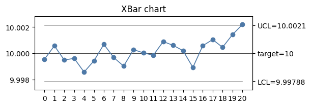
This example shows a point that violates the limit of an XBar chart (the data is here, the chart is shown in the section Control charts below).
mean_hist = 10.0
std_hist = 0.002
params = mqr.spc.XBarParams(mean_hist, std_hist)

# Load sample data (which is in-control)
df = pd.read_csv(mqr.sample_data('spc.csv'))
# Add an out-of-control point
df.loc[len(df)] = [10.0019, 10.0027, 10.0038, 10.0036, 9.9973, 10.0037, 10.0028, 10.0017]

statistic = params.statistic(df)
rule = mqr.spc.rules.limits()

alarms = rule(statistic, params)
alarms.tail()
16    False
17    False
18    False
19    False
20     True
dtype: bool
Combining rules#
MQR provides a mechanism (mqr.spc.rules.combine) to build more complex alarm logic from simple elements.
Any number of alarms can be combined with a logical operator to produce a new alarm.
More information and examples are in the API Reference.
This example creates a rule that triggers an alarm when
the statistic is less that the LCL or greater than the UCL, or
the statistic has 3 of 4 consecutive points greater than 2 standard deviations from the target, or
the statistic has 5 values either monotonic increasing or monotonic decreasing.
rule = mqr.spc.rules.combine(
    np.logical_or,
    mqr.spc.rules.limits(),
    mqr.spc.rules.aofb_nsigma(3, 4, 2),
    mqr.spc.rules.n_trending(5)
)
This rule is the same, except that it triggers an alarm only when all three of those conditions are true at the same time.
rule = mqr.spc.rules.combine(
    np.logical_and,                     # AND instead of OR
    mqr.spc.rules.limits(),
    mqr.spc.rules.aofb_nsigma(3, 4, 2),
    mqr.spc.rules.n_trending(5)
)
Custom rules#
Any function that has the signature
Callable(ControlStatistic, ControlParams) -> pandas.Series[bool]
can be used as an alarm rule. All custom defined rules with this signature will work with the combination functions, and will work with the plotting routines. All pre-defined control rules are defined as functions. The control rules are defined here, for reference: .
Note that the index of the output series must match the index of the ControlStatistic argument.
Control charts#
To plot ControlStatistics against ControlParameters, use mqr.plot.spc.chart.
This chart shows the sample data from Alarm rules above.
with Figure(6, 2) as (fig, ax):
    mqr.plot.spc.chart(statistic, params, ax=ax)
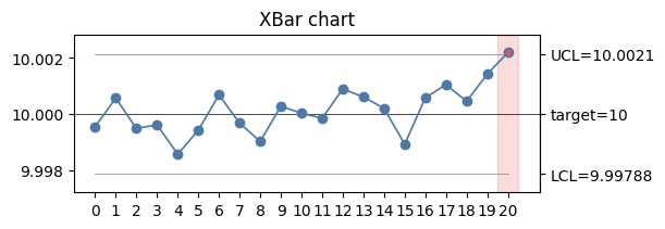
Alarm rules are shown as an overlay on the statistic.
The overlay shows a red point and a red-shaded region over the statistic plot.
The last point in the example above triggers an alarm according to the limits rule.
rule = mqr.spc.rules.limits()

with Figure(6, 2) as (fig, ax):
    mqr.plot.spc.chart(statistic, params, ax=ax)
    mqr.plot.spc.alarms(statistic, params, rule, ax=ax)
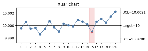
The same data will trigger the n_trending(4) rule.
This example demonstrates that only the last of the points in a violating subset is highlighted.
rule = mqr.spc.rules.n_trending(4)

with Figure(6, 2) as (fig, ax):
    mqr.plot.spc.chart(statistic, params, ax=ax)
    mqr.plot.spc.alarms(statistic, params, rule, ax=ax)
See more examples in mqr.spc.rules.
Historical vs. live data#
ControlParams represent the target and limits of an in-control process. Ideally, ControlParams should be created from historical or reference values for the process. For example, XBarParams would be created from an historical process target and standard deviation directly. That is true for all the types: the class attributes are the reference parameters.
mqr.spc.XBarParams(4.3, 0.21)
XBarParams(centre=4.3, sigma=0.21)
To create reference parameters from historical samples, use the .from_data methods, like this.
data = pd.read_csv(mqr.sample_data('spc.csv'))
mqr.spc.XBarParams.from_data(data)
XBarParams(centre=np.float64(10.000053750000001), sigma=np.float64(0.0018739437029978527))
Caution
The .from_data methods can be used to create ControlParams from live data,
but be aware that the limits are then 3\(\sigma\) (by default) from the mean of the live data.
As a result, the live data will rarely (about 0.03% of points, since the data were assumed to be normal)
trigger an alarm on its own limits.
ControlParams should only be created this way if the process is known to be in-control.
ControlParams can also be created from the statistics of historical samples. For example, RParams can be created from an historical sample range like this.
mqr.spc.RParams.from_range(2, nobs=5)
RParams(centre=2, sigma=np.float64(0.8598714945002754))
The resulting RParams has a target sample range of 2, and is parameterised on a process standard deviation of \(\sigma \approx 0.86\), which was calculated from the sample range. If the process standard deviation is known, use it directly:
mqr.spc.RParams(2, 0.86)
RParams(centre=2, sigma=0.86)
Saving ControlParams#
After ControlParams have been created they can be serialised to disk/file in two ways.
Use python’s
picklelibrary to serialise the object to an efficient binary format. Pickle data contains enough information to recreate the object directly, with no further type information.Use
mqr.spc.ControlParams.asdictto serialise the object to a dict and then JSON. The object can be recreated by passing the resulting dictionary to the corresponding constructor.
This is an example of pickling and then reconstructing an instance of RParams.
import pickle

params = mqr.spc.RParams(2, 0.86)
params_bin = pickle.dumps(params)
obj = pickle.loads(params_bin)

vstack(
    params_bin,
    obj,
)
b'\x80\x04\x95]\x00\x00\x00\x00\x00\x00\x00\x8c\x13mqr.spc.lib.control\x94\x8c\x07RParams\x94\x93\x94)\x81\x94}\x94(\x8c\x06centre\x94K\x02\x8c\x05sigma\x94G?\xeb\x85\x1e\xb8Q\xeb\x85\x8c\x06nsigma\x94K\x03\x8c\x04name\x94\x8c\x01R\x94ub.'
RParams(centre=2, sigma=0.86)
This is an example of serliasing to JSON then reconstructing the same instance of RParams.
import json

json_str = json.dumps(params.asdict())
params_dict = json.loads(json_str)
obj = mqr.spc.RParams(**params_dict)

vstack(
    json_str,
    params_dict,
    obj,
)
{"centre": 2, "sigma": 0.86, "nsigma": 3, "name": "R"}
{'centre': 2, 'sigma': 0.86, 'nsigma': 3, 'name': 'R'}RParams(centre=2, sigma=0.86)
Note that there is not enough information in the JSON representation to know which type is being constructed. Usually, the JSON will be stored in a way that makes it clear how it should be reconstructed. That is, the JSON will be stored at a location that contains only RParams, or the type name (“mqr.spc.RParams”) could be stored as metadata with the JSON.
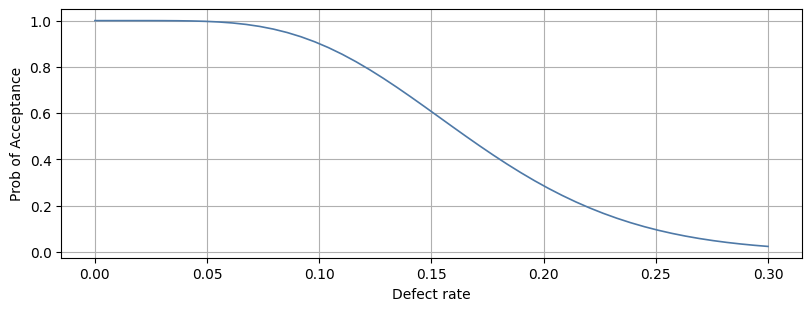
Acceptance Sampling#
AQL and LTPD conformance#
Detailed examples of AQL and LTPD calculations are given in: nklsxn/mqr-guide.
OC curves#
An OC-curve can be constructed using mqr.plot.spc.oc:
with Figure(8, 3) as (fig, ax):
    mqr.plot.spc.oc(n=40, c=6, defect_range=(0, 0.3), ax=ax)