Measurement System Analysis#
- Related modules
mqr.msa(andmqr.plot.msa)- Detailed examples
MQR can automatically configure an ANOVA to perform a crossed GRR study. Data should be arranged in a DataFrame with columns for the measurement, part identifier and operator identifier. These columns can have any names, which will be configured in the next step. The DataFrame can have other columns too, which will be ignored.
data = pd.read_csv(mqr.sample_data('grr.csv'))
data.head()
| Part | Operator | Height | |
|---|---|---|---|
| 0 | 1 | 1 | 9.347 |
| 1 | 1 | 1 | 9.230 |
| 2 | 1 | 1 | 9.202 |
| 3 | 1 | 2 | 9.365 |
| 4 | 1 | 2 | 9.423 |
Setting up a study#
Define the following parameters:
tolerance,
study variation,
column name mapping.
MQR uses the column name mapping to configure the GRR regression.
usl = 10.5
lsl = 7.5
tol = usl - lsl
sv = 6.0
include_interaction = True

name_mapping = mqr.msa.NameMapping(
    measurement='Height',
    part='Part',
    operator='Operator')
Construct the GRR study using mqr.msa.GRR.
The result is shown in notebooks as a table that summarises the inputs,
and shows the formula that MQR passed to statsmodels to calculate the regression.
grr = mqr.msa.GRR(
    data,
    tolerance=tol,
    names=name_mapping,
    include_interaction=include_interaction,
    nsigma=sv)
grr
| Measurement | Part | Operator | |
|---|---|---|---|
| Variable | Height | Part | Operator |
| Count | 90 | 10 | 3 |
| Replicates | 3 | ||
| Tolerance | 3.0 | ||
| Nσ | 6.0 | ||
| Formula | Height ~ C(Part) + C(Operator) + C(Part):C(Operator) | ||
Checking the regression model#
Use the regression result (GRR.regression_result) to analyse the model fit.
The tools from mqr.anova show a summary of the contrasts and the adquacy of the fit.
The residuals can be reviewed as demonstrated in Analysing residuals.
In the summary below, the interaction is not significant, and the GRR should be re-run without it. This example continues with the interaction included.
result = grr.regression_result

with Figure(5, 4, 2, 2) as (fig, ax):
    mqr.plot.regression.residuals(result.resid, result.fittedvalues, axs=ax)
    plot = mqr.nbtools.grab_figure(fig)

vstack(
    mqr.anova.adequacy(result),
    plot,
    mqr.anova.summary(result),
)
| S | R-sq | R-sq (adj) | F | PR(>F) | AIC | BIC | N | |
|---|---|---|---|---|---|---|---|---|
| 0.04256 | 0.9684 | 0.9531 | 63.43 | 0.000 | -289.3 | -214.3 | 90 |

| df | sum_sq | mean_sq | F | PR(>F) | |
|---|---|---|---|---|---|
| C(Part) | 9 | 3.211 | 0.3568 | 197.01 | 0.000 |
| C(Operator) | 2 | 0.08652 | 0.04326 | 23.89 | 0.000 |
| C(Part):C(Operator) | 18 | 0.03352 | 0.001862 | 1.03 | 0.444 |
| Residual | 60 | 0.1087 | 0.001811 | nan | nan |
| Total | 89 | 3.44 | 0.03865 | nan | nan |
Analysing results#
The variance table can be shown by constructing the type mqr.msa.VarianceTable.
mqr.msa.VarianceTable(grr)
| VarComp | % Contribution | StdDev | StudyVar (6.0*SD) | % StudyVar | % Tolerance | |
|---|---|---|---|---|---|---|
| Gauge RR | 0.003208 | 7.522 | 0.05664 | 0.3398 | 27.43 | 11.33 |
| Repeatability | 0.001811 | 4.247 | 0.04256 | 0.2553 | 20.61 | 8.512 |
| Reproducibility | 0.001397 | 3.276 | 0.03738 | 0.2243 | 18.1 | 7.475 |
| Operator | 0.00138 | 3.236 | 0.03715 | 0.2229 | 17.99 | 7.43 |
| Operator*Part | 1.699e-05 | 0.03984 | 0.004122 | 0.02473 | 1.996 | 0.8244 |
| Part-to-Part | 0.03944 | 92.48 | 0.1986 | 1.192 | 96.17 | 39.72 |
| Total | 0.04265 | 100 | 0.2065 | 1.239 | 100 | 41.3 |
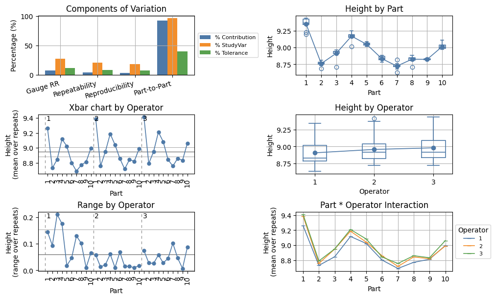
A graphical representation of the GRR study can be displayed using mqr.plot.msa.grr.
with Figure(10, 6, m=3, n=2) as (fig, axs):
    mqr.plot.msa.grr(grr, axs)